After a new project is loaded in ggKbase, a metagenome bin is created to contain all the unbinned genomes. In order to identify individual organisms from the metagenome bin, we use the binning tool to group contigs of genes based on their coverage, GC content, and phylogeny. This tutorial uses the Borehole JP project to demonstrate the binning process.
Step 1: Project / Organisms Page
From the Projects page, select the project that you want to bin. To follow along this tutorial, you will select BJP_08E140C01, which takes you to the organisms landing page: BJP_08E140C01 Organisms.
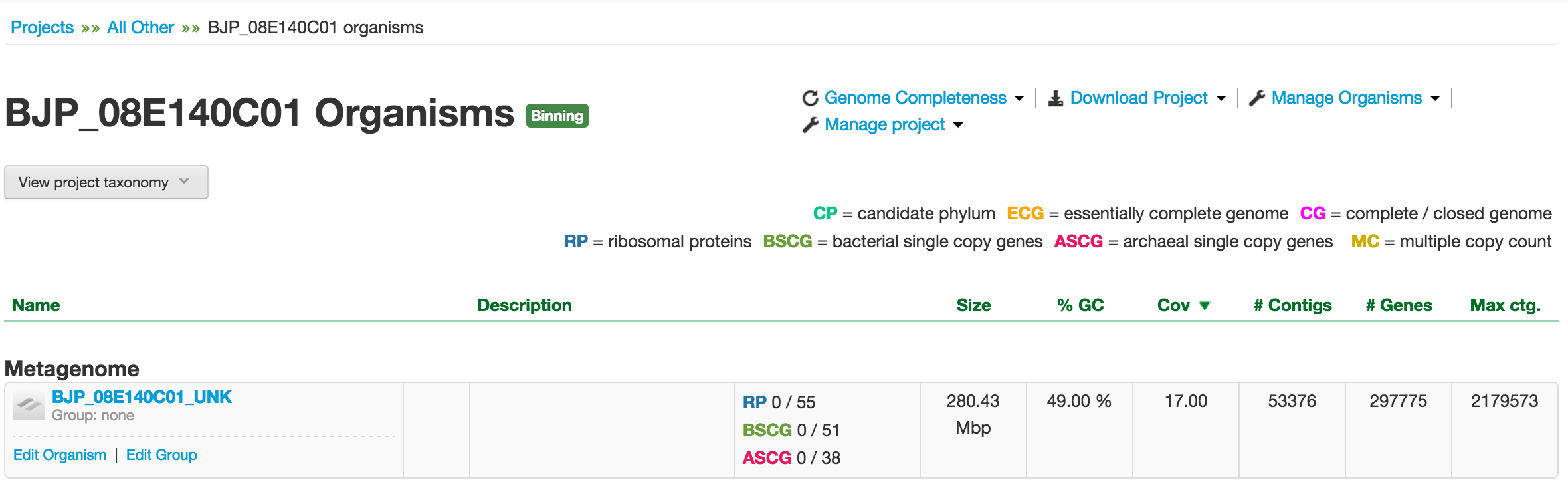
Metagenome organism landing page and its table of properties.
Since this project has not been binned yet, you should see only one “organism” in the Metagenome table. Note that the metagenome bin always ends with the suffix *_UNK to denote that the genomes in this bin are unknown. The table contains the name of the metagenome bin (linked to its metagenome organism page), its description, size, %GC, average contig coverage, number of contigs, number of genes, and the size of the largest contig. Right below the metagenome name, you have two links – Edit Organism and Edit Group – tools for editing its meta information.
To take a quick look at what the phylogenic composition of this metagenome bin, you can click on the “View project taxonomy” button.
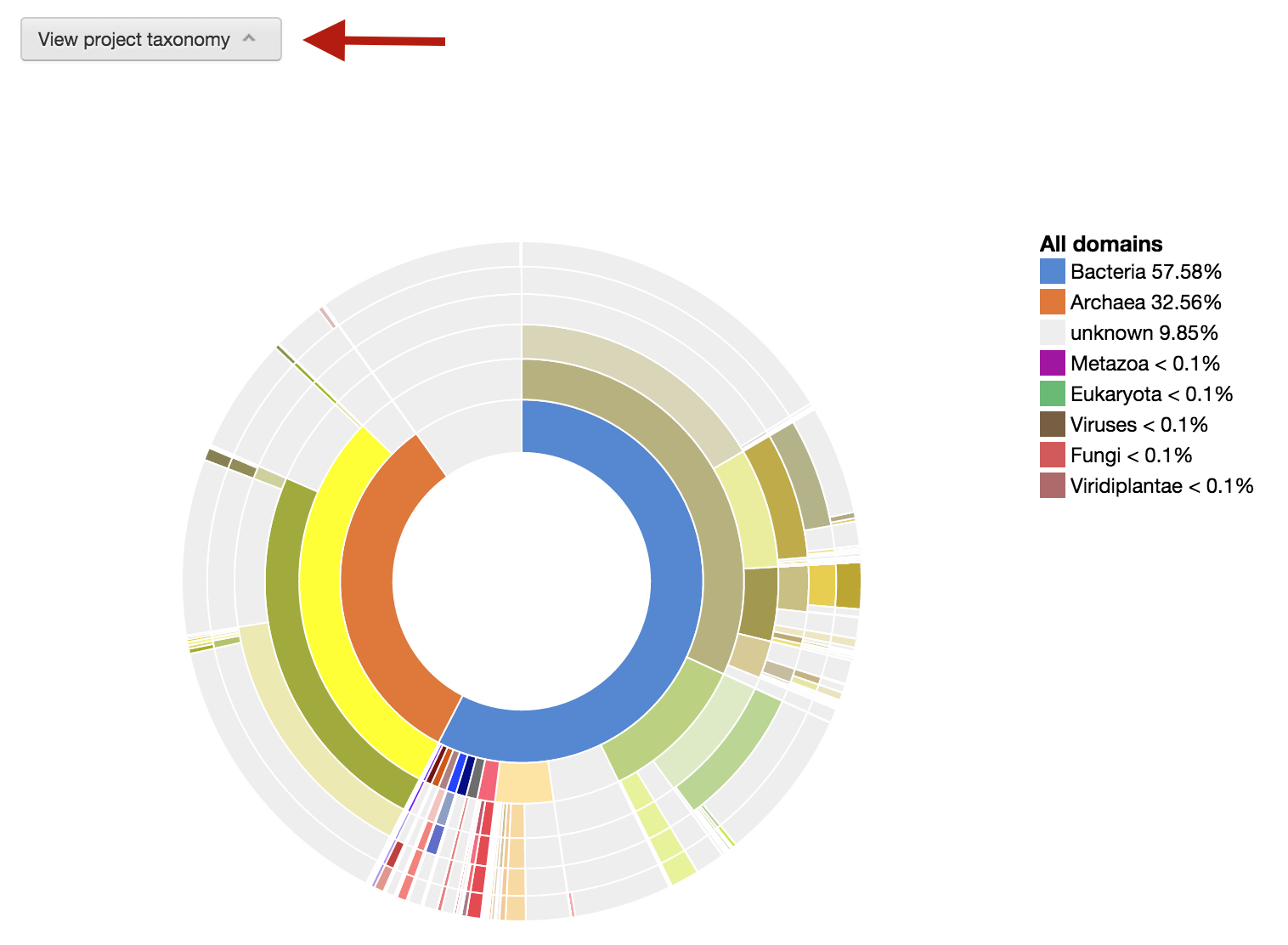
Phylogenic wheel for the metagenome bin.
Step 2: Metagenome Organism Page
Click on the metagenome bin [BJP_08E140C01_UNK] to open the metagenome organism page. The row of boxes right below the page title show the organism’s metagenomic context, taxonomy, properties, and genome completeness.

Meta information grouped in four categories.
The row of tabs contains a paginated list of the organism’s contigs, separate paginated lists for the different types of features (genes, rRNAs, tRNAs), a histogram and table of the ribosomal proteins, the bacterial SCG (single copy genes), the archaeal SCG, and lastly, a table of the taxonomic breakdown of each scaffold.
Lists of genomic data in tabular format.
![]() To start binning the metagenome, click on the Binning Tools link, located to the right of the page title. Note: After you have selected Binning Tools, it may take a little time for this page to appear if your dataset is large.
To start binning the metagenome, click on the Binning Tools link, located to the right of the page title. Note: After you have selected Binning Tools, it may take a little time for this page to appear if your dataset is large.
Step 3: Binning Tools
On the Binning Tools page, you are provided with 3 interactive controls (phylogeny wheel, GC content, and coverage) and 4 feedback signals (bacterial SCGs, archaeal SCGs, ribosomal proteins, a list of selected contigs, and bin summary stats). The three controls, which interact with one another, serve as filters to bin out individual genomes. The four feedback signals indicate the quality of the binning results.
Control: Phylogeny wheel
This is an interactive visualization for the phylogenetic composition of the metagenome at different levels of taxonomy. The scaffolds have been classified taxonomically based on the consensus phylogeny of 50% or greater of their respective genes. For more information about how the phylogenetic makeup of each scaffold is determined, click here.
To use it, you can click on any part of the phylogeny wheel to focus on one phylogeny, effectively filtering out undesired phylogenies.
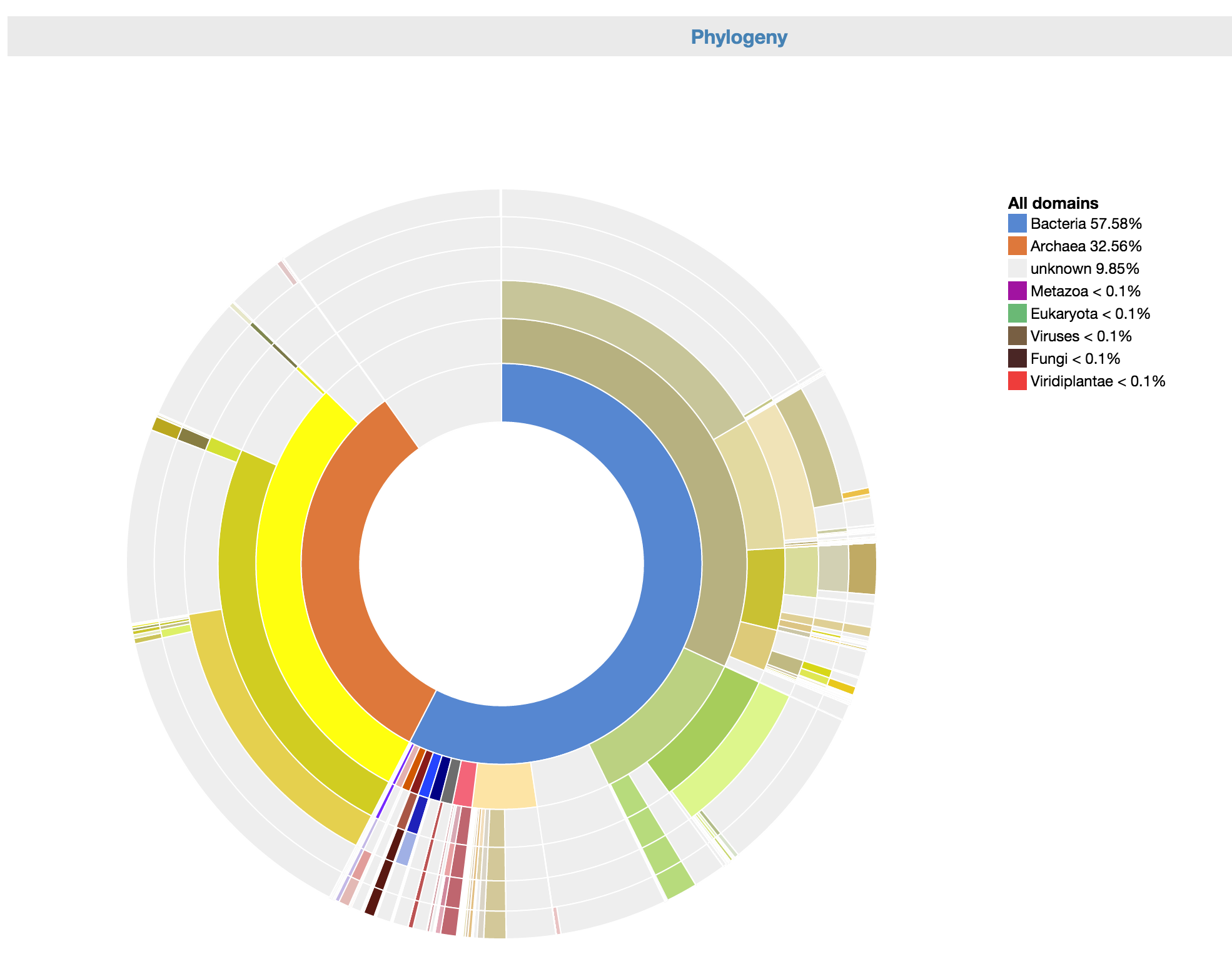
Control: Phylogeny wheel allows you to focus on a particular phylogeny.
Control: GC Content
The GC content can serve as a genomic signature. You can select a range of interest and view the taxonomic makeup of that fraction (above) as well as the coverage and SCG inventory (below). You may use the Min and Max GC input boxes to fine tune your selection.
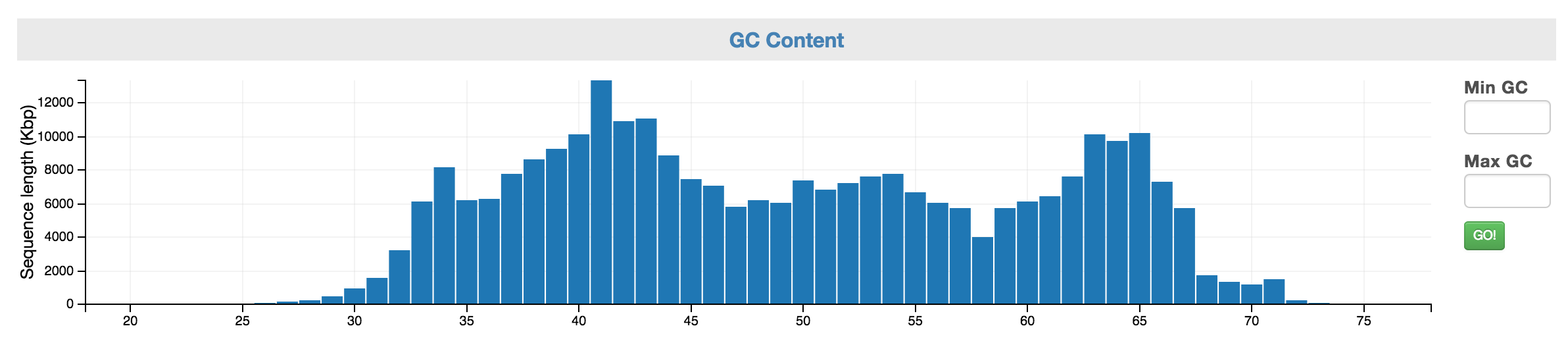
Control: GC Content allows you to select a range of GC content.
Control: Coverage
You can first narrow to a coverage range of interest using the “Zoom Coverage” chart on the bottom. And then, you can select the scaffolds using the top chart. You may use the Min and Max Cov. input boxes to fine tune your selection.
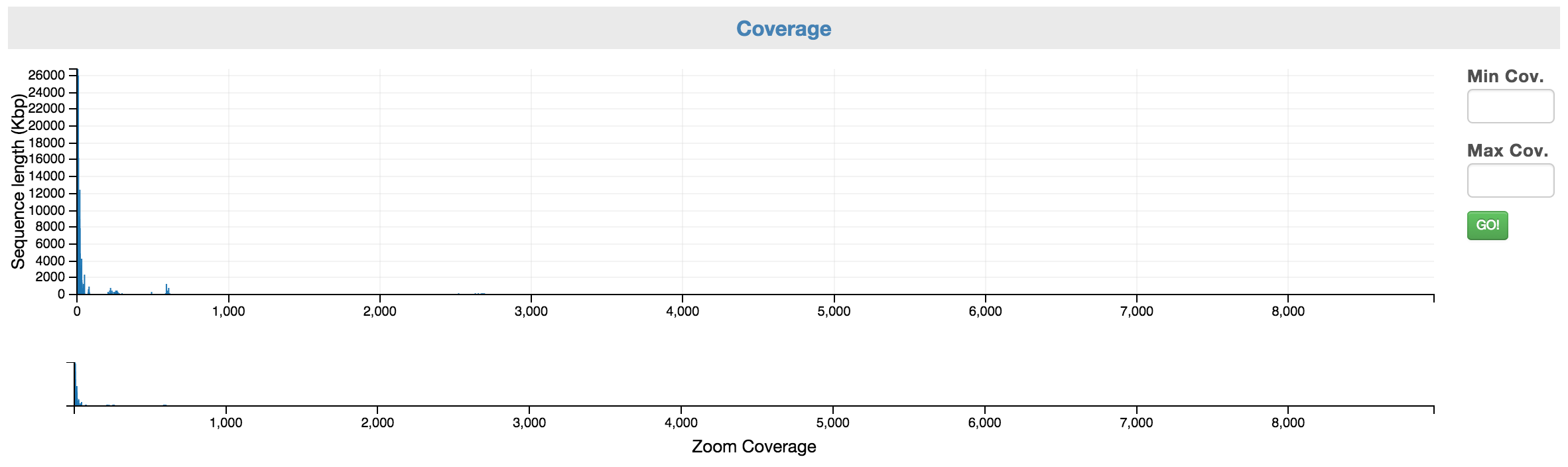
Control: Coverage allows you to select a range of coverage.
Here is how it looks like after you have narrowed the range of selection by highlighting a portion of the zoom coverage. Note: no scaffold has selected until you have highlighted the scaffolds on the top chart.
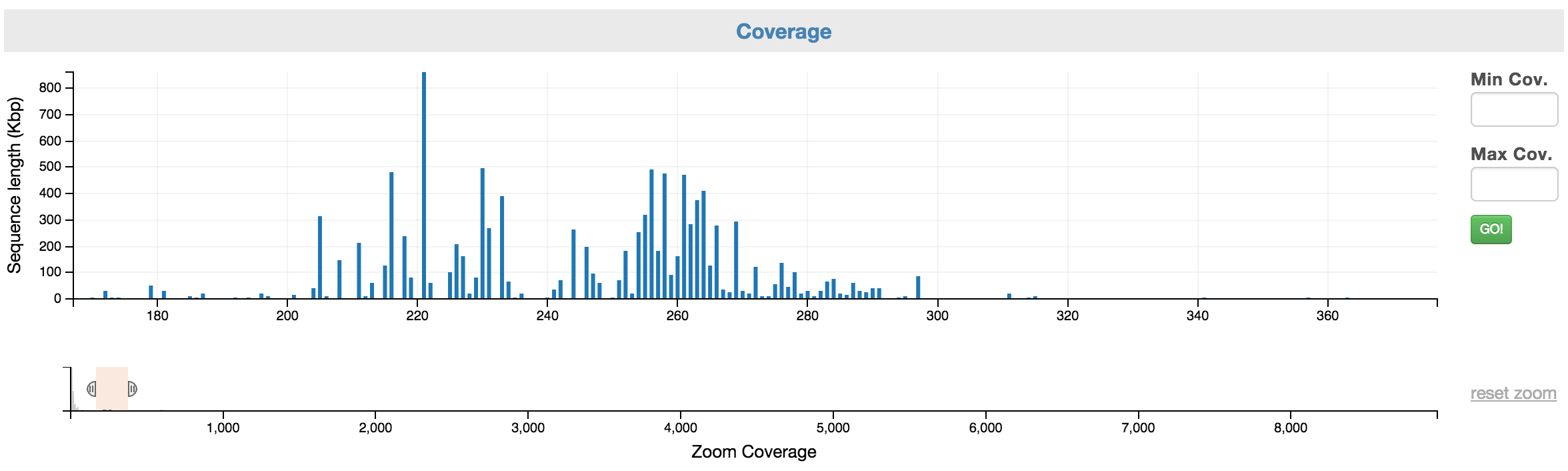
What the coverage selection chart looks like after it’s zoom range is narrowed.
Feedback: Bacterial SCGs. This displays bacterial SCG inventory of the unbinned data. A complete bacterial genome should ideally have one copy for each of the bacterial single copy genes.
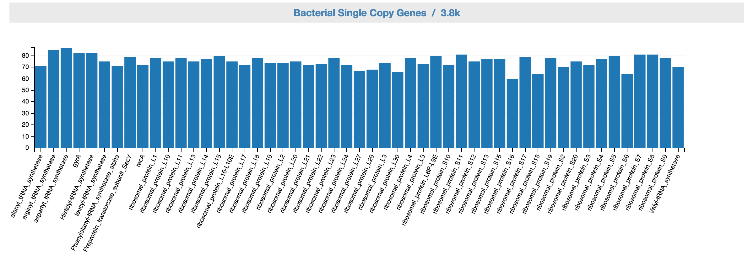
Feedback: Bacterial SCG inventory based on the controls.
Feedback: Archaeal SCGs
This displays archaeal SCG inventory of the unbinned data. A complete archaeal genome should ideally have one copy for each of the archaeal single copy genes.
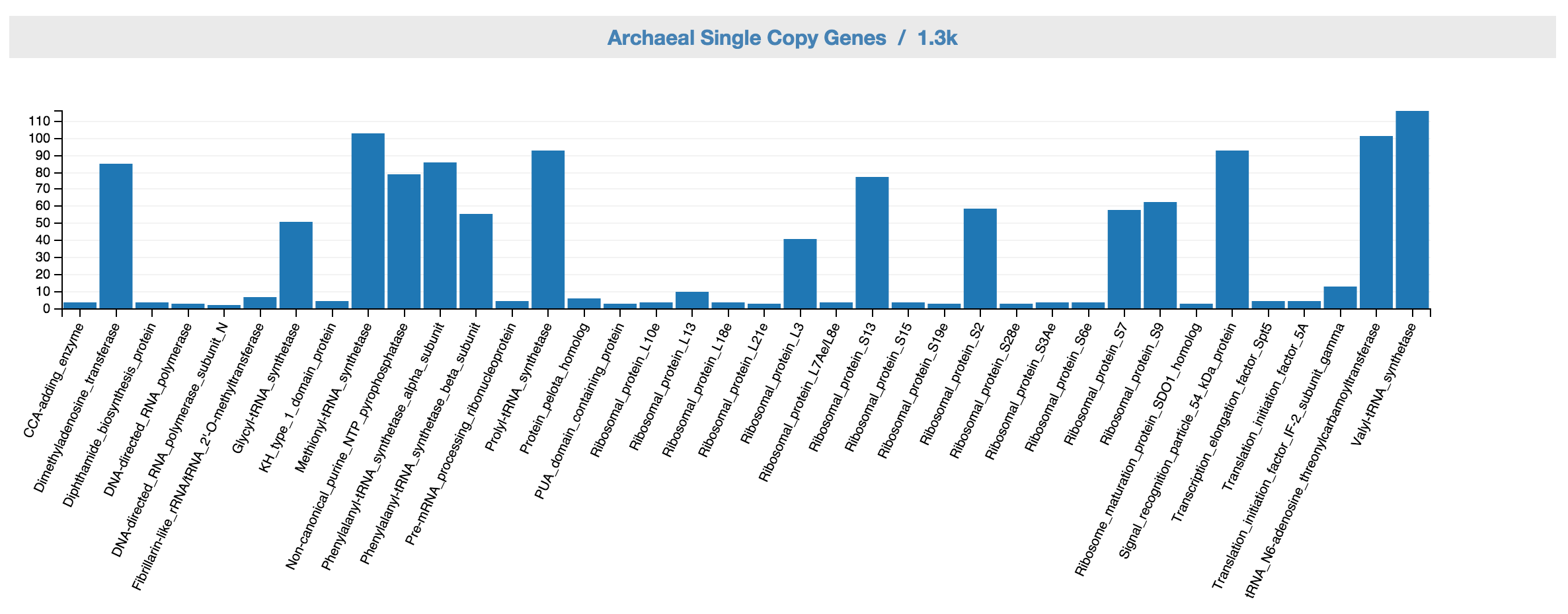
Feedback: Archaeal SCG inventory based on the controls.
Feedback: Ribosomal proteins
This displays ribosomal proteins inventory of the unbinned data. A good bin would have one copy of gene for each ribosomal protein.
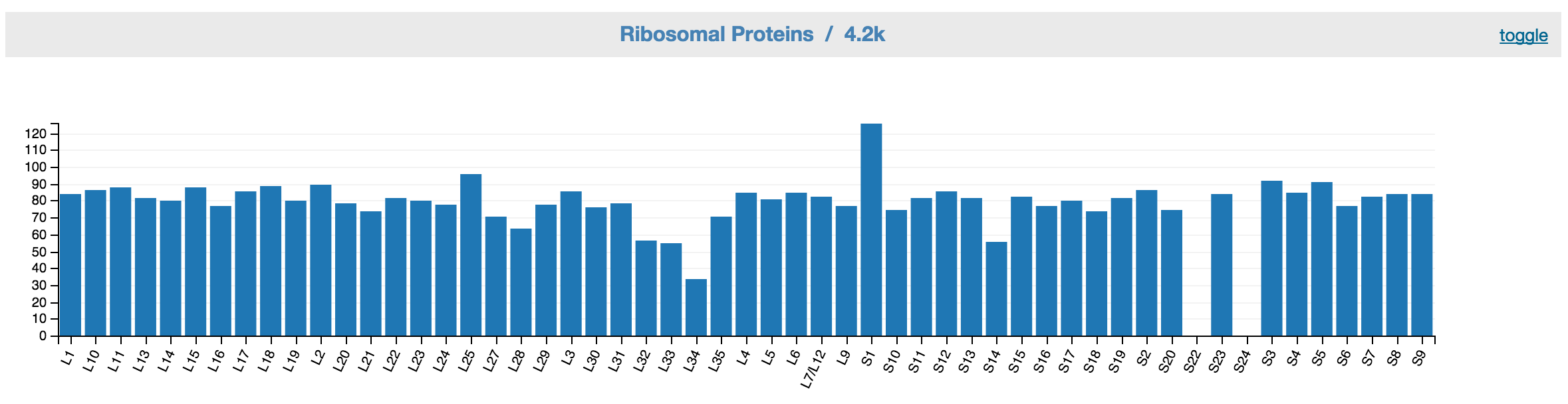
Feedback: Ribonsomal proteins inventory based on the controls.
Feedback: Bin summary stats
Once the controls are set, you are provided with the summary stats for the bin, which is located right below archaeal SCG graph. The summary displays the total sequence length of all currently selected contigs, their average GC content, average coverage and the total number of ribosomal proteins and single copy genes.
Feedback: Bin summary stats.
Feedback: Selected scaffolds
In addition to the bin summary stats, a list of scaffolds is listed. If you need to bin very precisely, you can examine each scaffold (right click on a link and open to a new tab/window) and verify whether the scaffolds belong to the bin. This is generally used in the last Step.
Feedback: A list of scaffolds selected based on the controls.
General Binning Workflow
- Typically, the best place to start binning is by identifying the high coverage organisms by using the Coverage control. Zoom into a high coverage range first and then select the scaffolds in that range.
- Define the GC range to exclude unwanted scaffolds.
- Use the phylogeny wheel to focus on the desired scaffolds.
- When the controls are set and the results are desirable, fill out the binning form as indicated by the comments below. Click on the Bin button.

Use the binning form to create a new bin.
Note: Because the controls influence one another as well as the feedback, you should examine the feedback results as well as iteratively adjust the other controls.
Step 4: Purifying Bin
To purify a bin by removing scaffolds that don’t belong to the bin (ex: a small amount of bacterial scaffolds are included a archaeal bin), you need to do the following:
- Open up the newly binned genome (or whatever bin you want to purify) and click on “Binning Tools” on the organism page.
- Use the phylogeny wheel to select the undesired portion of the wheel. Such selection would result in a list of scaffolds on the bottom of the page.
- Go through the scaffolds to figure out which ones are undesired, i.e. of a different phylogeny. You can take advantage of the phylogeny color.
- Once the undesired scaffolds are identified, click on “Manage this Contig” on the scaffold page, select “Rebin.”
- In the Rebin dialogue box, move the scaffold back to the metagenome bin.
1 thoughts on “Binning Tools and Procedures”
Comments are closed.